Overview
Typical uses
Importing data
Body types
Interactive interface
Forward and inversion modelling
Overview
Potent is a Windows application that provides a highly interactive framework for 3-D modelling of magnetic and gravity data.
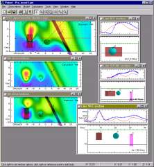
This example uses one of Geosoft's Oasis montaj sample datasets. The top left window shows the entire TMI dataset as a grid. The bottom left window shows the subset of data around the two anomalies of interest. The top right window shows an ENE section across this region. The anomalies have been modelled as a dyke and a flat tabular structure. The blue crosses are the observed TMI field, and the red line is the calculated field due to the model. The bottom right window shows the calculated field due to the model as an image at the same colour stretch as the observed field.
Potent works in 3-D space. Observation points can have height and ground clearance associated with them. The bodies that constitute the model are all able to be translated and rotated in three dimensions.
The field due to the model is calculated at the true position of the observations, thereby incorporating elevation effects such as those due to topography or aircraft height.
Top
|
(Click on an image to display an
enlarged version in a new window)
|
Typical uses
Potent is used for:
- Detailed orebody modelling for mineral exploration. Potent is used by mining and exploration companies.
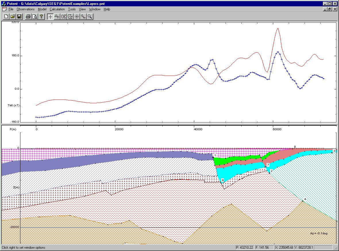
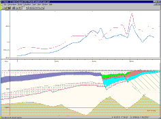
- Stratigraphic and structural modelling, such as for petroleum exploration and regional studies (see example opposite). Potent is an economical, versatile and highly interactive tool for building complex layered structures.
- Education. Potent is used by universities around the world for teaching potential field interpretation.
- Environmental and ordnance work. Potent is used for industrial decontamination studies and to help locate unexploded ordnance.
Top
|
|
Importing data
Potent can import observed data from ASCII files (such as Geosoft XYZ format files) and from Geosoft or ERMapper grids. Typical data sources include:
- Airborne surveys
- Regional gravity surveys
- Detailed ground surveys
- Down-hole surveys
- Any combination of the above
All datasets can be multi-component. Different types of data can be combined in the one workspace, allowing true multi-component, multi-dataset forward and inversion modelling.
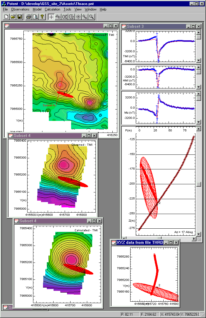
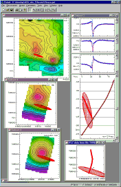
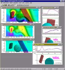
This example shows a lens-like interpretation (ellipsoid) for combined ground magnetic (TMI) and down-hole (multi-component) data. The top left window is the complete ground survey. The two below it show the observed and calculated fields of the subset of data around the anomaly of interest. The right-hand windows show the hole in cross-section (top) and plan (bottom). During inversion, the down-hole observations were weighted to make them more significant, hence the good fit of the down-hole profiles relative to the ground survey images.
Top
|
|
Body types
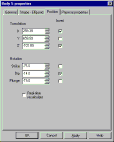
The following links display PotentQ, rather than Potent, screen snaps of the various body types. Potent body definitions are identical, but the bodies can be displayed as solid rendered as well as wireframe (as depicted in the image shown opposite, which includes all body types).
Bodies may be arbitrarily translated and rotated using the same Position dialog box in each case. (Bodies are usually moved by dragging with the mouse on plan and cross-sction windows, but can be positioned explicitly using the dialog box if required.)
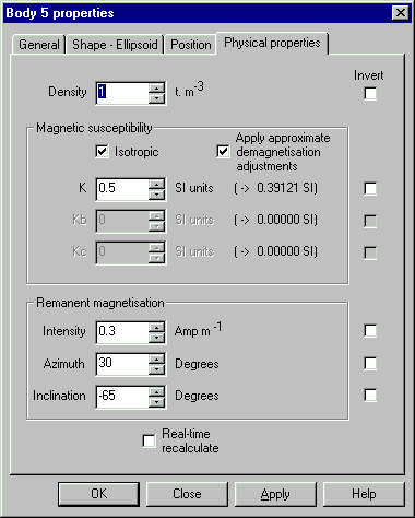
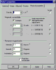
The magnetic properties of all bodies can include remanent magnetisation and anisotropic susceptibility. By default, magnetisation is induced and isotropic. Demagnetisation corrections are applied when feasible, depending on the body geometry.
Top
|

|
Interactive interface
Subsets and views
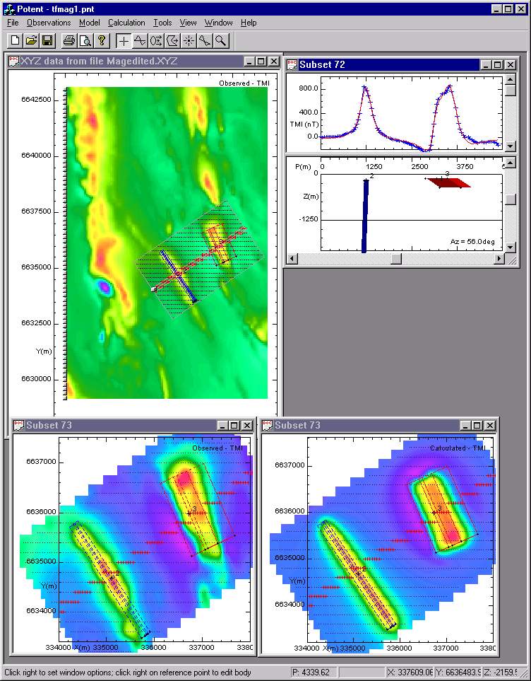
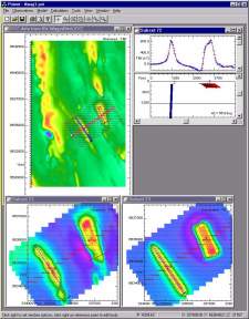
Potent allows you to create any number of subsets of your main datasets, and to display them in any combination of plan and cross-section ("profile") windows. This is demonstrated in the example opposite, which shows two subsets taken from the point-located TMI data (shown in gridded form for convenience) in the top left window. (Click on the image to see a full-size version.)
The bottom two "plan" windows are both of subset 73, which consists of data enclosed in the rectangular area shown by blue dots in the main data window. One plan window shows the observed field, and the other the calculated field.
The top right "profile" window is of subset 72, which consists of data sampled from the flight lines along a narrow rectangular area (red crosses on the main window).
Real-time calculation
By default, Potent recalculates automatically whenever you complete an operation (such as dragging a body) that affects the calculated field. Profiles are redrawn and grids of calculated and residual fields are re-gridded to reflect the change.
The "dynamic calculation" mode ("off" by default) causes Potent to calculate and redraw as changes are being made to a body, effectively animating the calculated field profiles. You can usefully activate this feature when the number of points to be calculated is not too large (less than 100 or so, depending on the computer and on which body type is being used).
Top
|
|
Forward and inversion modelling
In Potent, forward modelling is implicit; changes to the model are automatically applied to calculated profiles and images.
Inversion modelling is based on the non-linear least squares method described by Jupp & Vozoff (Geophysical Journal of the Royal Astronomical Society, vol 42, 1975). The implementation is versatile and, in its simplest form, very easy to apply. There are two steps:
- Create and display one or more subsets that include the observations that you want to include in the inversion. Minimise or close all other subset windows.
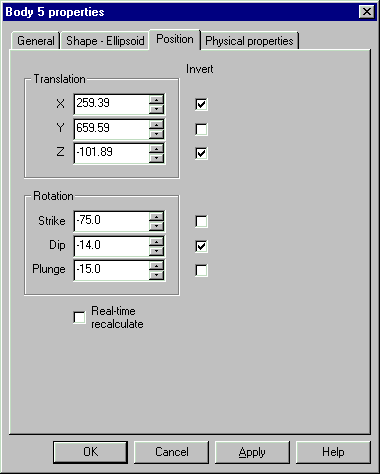
- In the dialog boxes for each body, check the "invert" checkboxes that correspond to the parameters that you want to be varied during the inversion. In this example the inversion will optimise the X coordinate, Z (the depth), and the dip. The other tabs of the dialog box (such as "Shape" and "Physical properties") might also have parameters that are marked for inversion. Similarly, other bodies of the model might also be optimised during the same inversion.
Once this is done you can start the inversion. The RMS error is displayed in the status bar at the bottom of the main Potent window at each iteration.
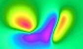
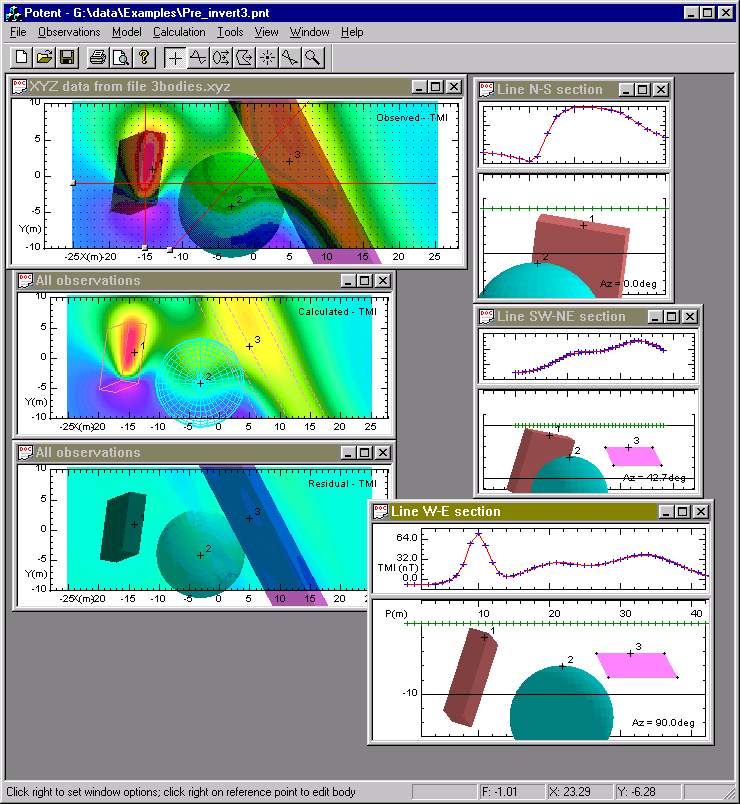
This example shows a three-body model before and after a 50 iteration inversion. The position (including orientation) and shape of each body was allowed to vary. Images of the observed, calculated and residual field are all shown with the same colour stretch.
Top |
|
| |
|
|